A Wrap Up on Water

This summer has certainly flown by! I cannot believe that my experience in Texas has come to an end and it is again time for classes at Cornell! I lookback on my experience and I cannot believe what I have learned! I have been exposed to many aspects of dairy farming on a large scale! From the operation of large equipment, to assisting during vet check; Introducing new technology on the farm to repairing broken irrigation equipment in the field. I feel that I have truly gained an adequate understanding for large-scale dairy operations and certainly a greater interest.


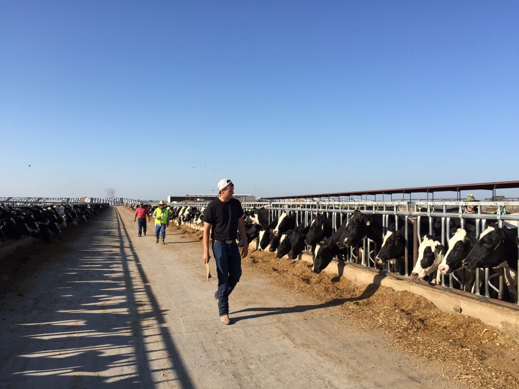
Walking the pens for Vet Check.

Walking the pens for Vet Check.

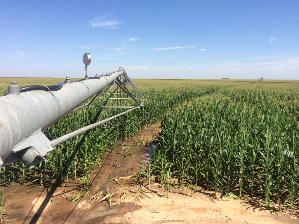
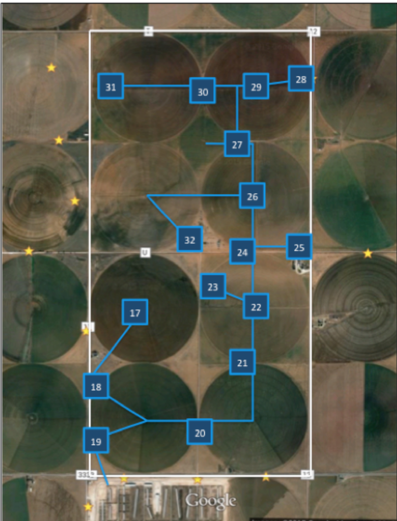
After the completion of my intern project I have found that there were 107 crop circles feed by 219 wells! This attests not only to the scale of the farm but also for their need for adequate irrigation. It is well known that water availability is arguably the most import resource in agriculture. However it has taken a drought half a decade long for much of the nation to realize the true scarcity of this essential component of life. My summer experience has open me to a new perspective on what agriculture might look like 30 years from now, and I ask myself… water we doing?

View over tasseling corn field.

View over tasseling corn field.

Example Map representing well locations and connecting water lines.

Example Map representing well locations and connecting water lines. This maps exemplifies the lack of ground water. 

Greenhouse Gas Emissions

As a member of the Nutrient Management Spear Program, I am assigned to a specific project with my field supervisor, but I, along with all interns, get involved in other projects happening within the Program. Cornell’s NMSP as well as various colleges and universities work collaboratively for the project “Dairy CAP” under the leadership of University of Wisconsin’s Dr. Matt Ruark. The NMSP’s part in Dairy CAP entails the greenhouse gas emissions project.

The objective of the NMSP’s greenhouse gas emission project is to quantify emissions from manure and compost, rate and timing for corn, and method of manure application (injected vs broadcast). Emissions were measured at Musgrave Farm in Aurora, NY on Field Z corn (5 replications, 50 plots total), alfalfa (6 replications, 24 plots total) and grass (6 replications, 24 plots total). In Field Z corn, there were organic and inorganic applications. For organic, phosphorus-based (P-based) and nitrogen-based (N-based) manure and compost was used. For inorganic, 0 lbs, 50 lbs, 100lbs, 150 lbs, and 200lbs per acre was used. N-based refers to the nitrogen needs as P-based refers to phosphorus needs

The three greenhouse gases (GHGs) measured in the project are carbon dioxide (CO2), methane (CH4) and nitrous oxide (N2O). CO2 is the least potent of the GHGs following CH4 (about 24 times more potent than CO2) and N2O (300 times more potent than CO2),  the most potent GHG.

We use only one method for obtaining GHGs from the fields. This is what the typical setup looks like at Field Z:

Emissions equipment in Field Z

Emissions equipment in Field Z

A frame is hammered into the ground with a hammer and a piece of plywood. This serves as a platform to place the chamber and create an enclosed environment to capture GHGs. Clips are used to further seal the frame and chamber together to prevent GHGs from escaping.

A syringe is used to collect the GHGs from the setup when the needle is placed through a nob at the top of the chamber. Before insertion, the syringe must be “closed” to avoid other gases from entering the syringe and contaminating the sample. Once the needle is in the chamber, the syringe must be “opened” before GHGs can be drawn out, but the syringe must be closed before the needle is taken out of the chamber to prevent losing any GHGs collected inside the chamber and contaminants from entering the syringe. The sample is injected into a vial and later analyzed in the lab.

Fellow intern, Andrew, drawing GHGs out of chamber via syringe.

Fellow intern, Andrew, drawing GHGs out of the chamber via syringe.

The collection of these samples takes place over an hour period. There are four “rounds” (T0, T1, T2, and T3) where 6 samples are collected from each replication in Field Z corn and 8 samples are collected from Field Z alfalfa and grass with the NMSP. Once the sampling begins in Field Z corn, there is a 2 minute interval between collecting each sample in each round, but in Field Z alfalfa and grass, each interval is 1.5 minutes since the chambers are closer together than chambers in Field Z corn.

We continuously sample from Field Z to determine when the greatest period of emissions occurs. Based from our findings, emissions appear the greatest after significant rainfall.

Summer Wrap Up

My plan for this last blog post is to fill in some missing details and provide a final reflection of my summer working for the Sustainable Cropping Systems Lab.

Over the course of the summer, I have been writing about specific experiments that I had been involved in. However, there were other projects that I was involved in. Early in the summer, our lab aided the Cornell small farm program on a tillage experiment. This project was very memorable for our lab because it involved transplanting 20,000 cabbages by hand over three days. The experiment was testing the effect of different combinations of tillage and above ground applications. There were three above ground applications: mulch, compost, and no application. The tillage treatments were different intensifications of tillage. While we were only involved in the three days of planting, after harvest I did get to have some of the cabbages.

IMG_2689

Over the course of the semester, I worked a lot with the Laurie Drinkwater Lab. I worked collecting biomass samples and processing samples for one of the Phd candidates, Emily Reiss. I also weeded plots for another grad student in the Drinkwater lab, Bryan Emmett.

Overall, I loved working for the Sustainable Cropping Systems Lab. Coming from a vegetable production background, I was able to learn so much more about grain production and cover crop management. I have also learned how a work environment can make a job. The Ryan Lab was made up of amazing people. As the leader of the lab, Matt Ryan, he set the tone. He emphasized how we should be using our time at the lab as a learning experience. Our lab manager, Chris, and research technician, Sandra, who we also called mom and dad, were incredible. They gave us the independence to work on certain projects. They answered so many of our questions and made the monotonous tasks fun. The grad students, Jeff Liebert, Margaret Ball, Connor Youngerman, Kiera Crowley, and Ann Bybee-Finley always made us feel appreciated which made coming to work every day that much better. In all, there were about 8 research assistants including myself. With so many different characters, it was a very entertaining summer. I think the combination of the people I was working with and the research we were involved in led me to gain a sense of pride in the lab and in my work.

11114176_1034384969906135_7410476405526646561_o


Lastly, I have enjoyed the summer so much that I will continue to work for the Cornell
Sustainable Cropping Systems Lab through the semester. I encourage anyone who has been interested in my summer work or who is interested in working for Matt Ryan’s Sustainable Cropping Systems Lab to contact me.

A Tangent on Potatoes

As a potato packer for Wegman’s Food Markets in the North East our family farm, Williams Farms, requires a constant supply of produce all year long. As a result potatoes are purchased from all over the US and Canada in order to be packed and redistributed to buyers in the North East. One of our sources for fresh potatoes during our off-season is Barrett Produce a packing shed also located in Muleshoe, Texas. So this weekend I decided to take a short break from dairy cattle and circles of corn to learn about potato production in the Panhandle of Texas.!


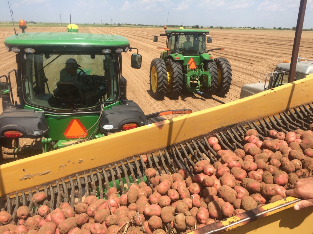
Most of the potatoes grown in the panhandle are either Reds or Russets and are grown on a sandy loam soil, as drainage and compaction are two important aspects of growing potatoes. A full circle of potatoes requires wells that can supply approximately 800 gallons of water a minute throughout an average growing year. The potatoes are harvested with a 4-row harvester, loaded on bulk truck and shipped up to 60 miles to be packed and distributed. The Barrett’s have limited storage capacity and as a result within two days after being dug, the potatoes have left the farms possession.


Additionally I was able to attend a variety field day hosted by the Barrett’s and the research team at Texas A&M. New varieties of mainly red and russet potatoes were displayed to growers all around Texas and other locations throughout the US and Canada. It was a great opportunity to ask additional questions about potato production in the Southwest and build my professional network!

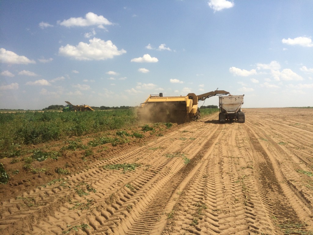
Trucks are pulled by tractor to ensure that they don't get stuck in the sand.

Trucks are pulled by tractor to ensure that they don’t get stuck in the sand.

Digging potatoes and loading them onto bulk trucks.

Digging potatoes and loading them onto bulk trucks.

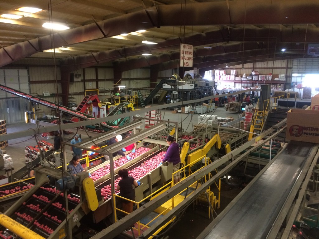
Packing facility

Packing facility

The last day of field work of my summer intern

Last Friday, Aug 21th, was my last day of field work of my summer intern. Amir, Greg and I went to Aurora Research Farm to collect green house gas sample in the corn field.

IMG_5411

It was a nice day to do field work, as the weather is not so hot and is not cold either, and on that day I finished my work quite smoothly, making no small mistakes.

IMG_5409

I remember that on the first day that I learned to do the collecting work, Amir instructed me very patiently, making sure that I understood every single step.

I also remember that there’s one extremely cold and windy day, Amir, Jeff and I worked in Aurora that day, and Jeff didn’t know it was such a cold day, and thus was still wearing his T-shirts and shorts, and he got a cold after that day’s work.

I also remember that there’re more than one day when it’s very dry in the field, and the soil became very compacted, so some bases of our chambers got out of the soil. Dennis, our hercules, hammered heavily on the wood board above the base, to put the base back to the soil.

This is the first summer I spend abroad in the US, it’s so lucky for me to have such a valuable chance to work in NMSP with these interesting and great people.

IMG_5415

At the end of the day, Amir and Greg were talking about the tall fescue grassland. They harvested the grassland just several days before, so the grassland seemed to be very flat. Amir said, I really like to look at the grassland in this direction, this is my favorite scenery. Greg said, yeah, it’s really nice, it looks like an airplane runway. A lot of people have worked in this “airstrip”, someone have left, someone is still working on it, and I hope everyone’s life and career can take off from here soon.


MERN calculation and the criteria to determine the optimum model when fitting

I wrote a blog post about the models used to fit the data of yield nitrogen fertilizer response in my winter cereal project:

https://blogs.cornell.edu/agsci-interns/?p=2918.

There are five models in it: quadratic model, exponential, square root, quadratic plateau and linear plateau model. However, the reason why we need to fit these models is that we need to calculate the MERN (Most Economic Rate of Nitrogen), and based on different models, the most MERNs are various.

  • The following is the general way to calculate the MERN:
Max(pY(N)-wN)

where N refers to the nitrogen fertilizer rate, Y(N) refers to the corresponding yield under that nitrogen fertilizer rate, p is the assumed unit price of dry biomass of forage yield, and w is the assumed unit price of the nitrogen fertilizer. Let

F(N)=pY(N)-wN

F(N) is maximized when the first derivative of F(N) equals zero, so

F'(N)=pY'(N)-w=0 

so that MERN is calculated by solving this equation:

Y'(N)=w/p
  • The necessity of selecting the optimum model:

an example of how MERNs are various based on different models, using the data from a site.

various MERN

The MERNs range from 94.23 to 68.52, and the yield at MERN ranges from 1.079 to 1.101 in this site, and the yield’s range can be much bigger in other sites. The diversity of MERNs suggests that in some cases, the farmers may apply too much nitrogen fertilizer using improper model, which would lead to the waste and pollution of N fertilizer, while in other cases, the farmers may apply too little nitrogen fertilizer using improper model, which would result in less yield of forage.

  • The criteria to determine the optimum model:

Traditionally, a lot of researchers tend to use the coefficient of determination to measure the goodness of these models, but many papers point out that in some cases, the R square of these models are very close and all high enough. For instance, if the R squares are 0.8543, 0.8678, 0.8462, 0.8514, 0.8401 respectively, there’s no significant difference between them, and they are all close to 1. It’s not a good idea to draw a conclusion of which is better directly from the coefficient of determination.

Similarly, some use criteria like root mean square error, residual mean square etc. , which have similar function and magnitude with R square.

In general, one important criterion to evaluate a regression model is its normality, and thus the normality of the residuals, which is the observed yield minus predicted yield based on the regression model, is regarded as a significant criterion in some paper.

residuals when fitting a square root model

In the plot above, the data of residuals are plotted with the corresponding nitrogen treatment. If the data point is above the x-axis, then the regression model tends to underestimate the yield, while if the point lies beneath the x-axis, then the model tends to overestimate the yield. Therefore, under the same treatment, when the data points lie symmetrically between two sides of the x-axis, the normality of the residuals are good enough, or the regression model has systematic bias.

deviation from mern

Also, after calculation of MERN, some use the nitrogen treatment deviation from MERN instead of nitrogen treatment as the x-coordinator. It has similar function, but focuses more on whether there’s any systematic bias around MERN.

In addition to using residual plots to visualize the goodness of the normality, some use Shapiro-wilk test to quantify the normality of the residuals. The null hypothesis of this test is that the population is normally distributed, so the more the p-value is close to 1, the better the normality is. Similarly, some others use Kolmogorov test to compare the normality, but this test is thought to be less powerful than Shapiro-wilk test.

Eventually, some would calculate the potential economic loss. The general steps of calculating potential economic loss are followed:

  • Assume that one model is the correct model, calculate the MERN and yield at MERN based on this “correct model”
  • Calculate the profit of the “correct model” by using the formula: (yield at MERN*price of forage)-(MERN*price of N fertilizer)
  • Calculate the profit of the other models by using the same formula. The MERN here is still based on the “correct model”, but the yield at MERN is calculated using the “incorrect models” to predict yield at MERN of “correct model”.
  • Calculate the difference between the profit between the “correct model” and the “incorrect models”.
  • Evaluate the risk of choosing the “incorrect models”.

Fun Work Days

As a part of my internship, I encountered many opportunities to attend agriculturally-related events as well as visit beef cattle farms in the Finger Lakes Region.

The first event I attended while working under the NMSP was the Cornell Seed Growers Field Day, where the topic of discussion focused on small grains and forages. Many speakers talked about the varieties of small grains and forages, all providing pros and cons for each option. Identification and prevention of disease and pests were other components of the seminars given at this field day.

The second event, the North American Manure Expo, was located in Chambersburg, PA. The morning was filled with seminars on manure application (specifically injection) and the benefits of injection. Tractors and manure application equipment lined the Expo grounds as well as exhibits with businesses, services and research projects for public display. Demonstrations for dry- and liquid-based manure ended the Expo, leaving the audience impressed with the liquid injection of manure.

Manure injection was the primary project I worked on this summer, so the event was an eye opening experience since it showed me how my research with NMSP was part of a bigger picture in the scheme of agriculture.

Manure Expo Demonstrations

Manure Expo Demonstrations

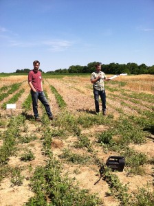
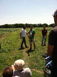
The Aurora Field Day at the Musgrave Research Farm encompassed most of the research I have conducted with the NMSP and encountered from other Cornell University research programs this summer. Many interns from other programs at Cornell participated in the trials happening at the research farm. Besides learning about all of the research happening at Musgrave, it was satisfying hearing my supervisors explain our greenhouse gas emissions, manure injection and green seeker projects I am a working on and, again, hearing the big picture concepts to our research.

Matt Ryan explains his research with cover crops

Matt Ryan explains his research with cover crops

Fellow intern, Isaac, demonstrates how Greenseeker equipment functions in Field Z

Fellow intern, Isaac, demonstrates how Greenseeker equipment functions in Field Z

I made three additional trips (with Quirine’s permission) based off my interests in beef cattle. Nancy Glazier, a Cornell Cooperative Extension small farms specialist, guided me through each event. The first beef-related trip I took part in was a monthly meeting where a group of experienced and inexperienced beef cattle farmers shared their financial struggles in starting up and maintaining beef cattle. I learned a great ordeal from the trip and met a great group of people, which set the stage for my next trip.

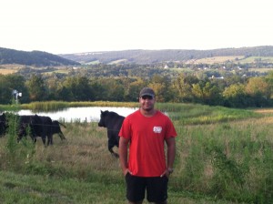
These black angus seem to dislike me

These black angus seem to dislike me

The following week Nancy took me on tours to multiple farms raising beef cattle, namely High Point Farm, Adventureland Devons, Just Serependity Farm, and Hidden Canyon Farm. Each location managed their herd with different methodologies and bases of knowledge, making each farm unique. With each visit I gained a lot of advice and support in raising beef cattle.

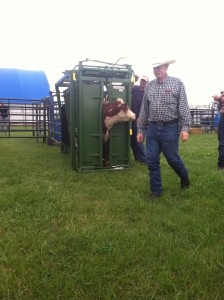
I traveled to Seneca Falls to check out the Empire Farm Days a week after my visits. Similarly to the Manure Expo, there was plenty of farm equipment and exhibits for display as well as seminars on cover crops and soil health. Here I watched Dr. Mike Baker demonstrate cattle handling and received my Beef Quality Assurance Certification (BQA). The required seminar for BQA was long and a test was administered. Following the test, we had to give a cow a subcutaneous injection. I never gave a subcutaneous injection before, so it was quite the experience and no harm was done to the animal.

Dr. Mike Baker shows his audience how the handling system functions

Dr. Mike Baker shows his audience how the handling system functions

MOSS (Musgrave Organic Soybean Silage)

  The last experiment I worked on was the Musgrave Organic Soybean Silage (MOSS) experiment. The head person on this project was a new grad student, Kiera Crowley. The experiment aims to compare different winter cereal management in corn and soybean rotation. The winter cereal used in all of the management experiments was cereal rye. There are four different winter cereal management’s being tested in this experiment: a no-till with the cereal rolled and crimped, a plow down, a management where the rye is cut for silage and what’s left gets plowed under, and a no cover crop management. Kiera plans on running multiple tests on the experiment to see if these different managements are having any effect. I helped execute soil property tests and water infiltration tests. In addition to that, Kiera is analyzing weed suppression and yield.

From the last post, you can see that I have done some soil sampling before. We took sixteen samples from each plot and there are twelve plots. We took these samples in order to analyze the soil properties. Bigger soil core samplers were used so we could examine aggregate stability. Four samples were taken from each plot. When taking the soil cores for aggregate stability, it was a more challenging and time-intensive process than regular soil sampling. The soil core had to be 6 inches and the diameter of the sampler was greater than 2 inches. In order to get the sampler down 6 inches, it took force and some finagling. After taking the sample out of the ground, we had to be careful not to disturb the soil too much. The test was for aggregate stability which is a factor of soil structure, so the less disruption of the soil structure, the better. All the soil was taken back to the lab for processing. The processing of the samples dealt with chemistry. I was able to help with some of the processing of the mineralizable carbon test. Kiera had done all of the prep work and my job was just to extract the mineralizable carbon.

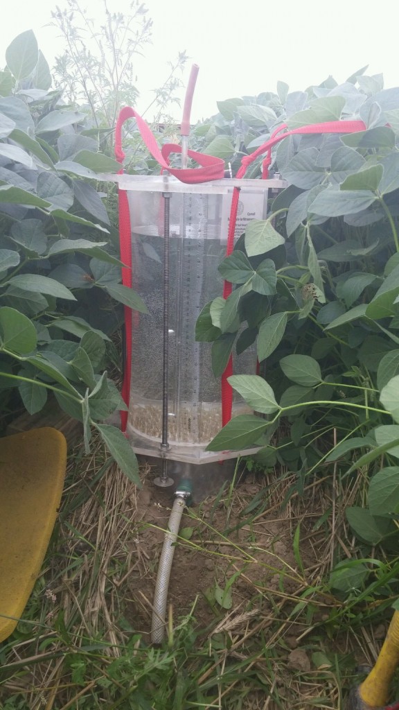
The second piece of the experiment I worked on was the water infiltration tests. The water infiltrometer is a device used to measure the water infiltration (the process by which water flows into the soil).

IMG_3005

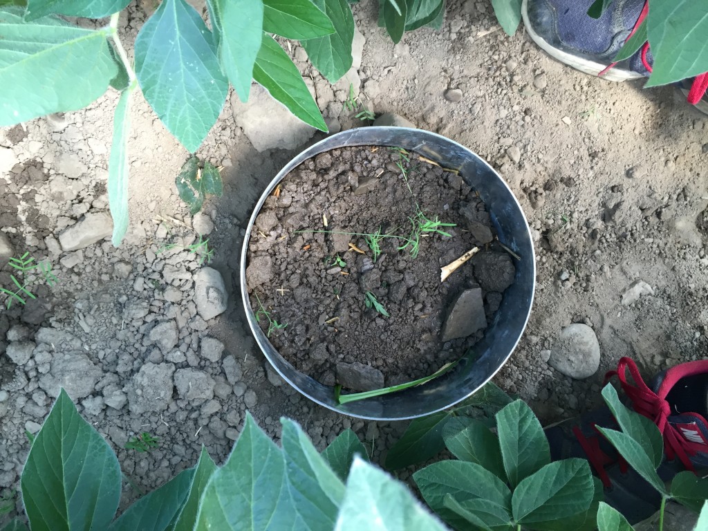
Base of the Infiltrometer

IMG_3006

Infiltrometer all ready to go

IMG_3003

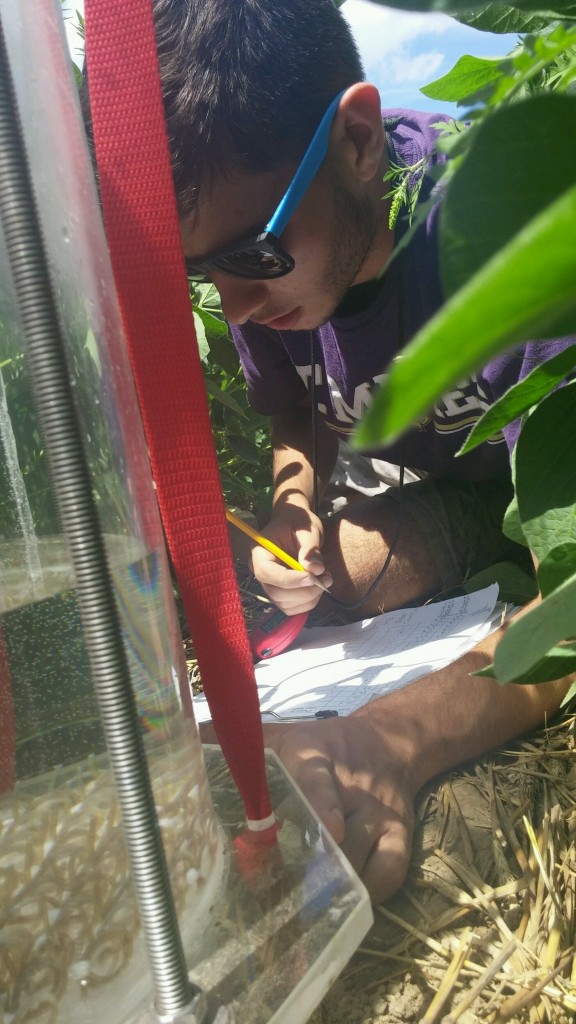
Recording results from Infiltrometer


Infiltrometers let you fix a rate of water dispersal onto soil. Infiltrometers can be used different ways depending on what you are looking for. We were interested in time until runoff. This involved recording the height of the water in the infiltrometer every minute. This way you can find the rate for each minute and can check to make sure it is staying consistent. This process is continued until there is runoff. After runoff had occurred, we recorded the amount of water that was used and the time it took to runoff. Working with the water infiltrometers was a very interesting and educational experience. The first time we tried to do water infiltration it didn’t go as planned. The rate is meant to stay consistent the whole time. While we had some successful infiltrations, during many of the infiltrations the rate kept decreasing and with some we never got runoff. We weren’t even able to finish all of the plots and this is very important because all of the samples should be taken within the same day. After some clarification and advice from a few people, we made some adjustments. The second time running the water infiltration tests were much more successful. The rates were staying consistent and we were able to finish within one day.

The models used to fit the data of yield nitrogen fertilizer response

As I’ve been working in the project that try to determine the optimum nitrogen rate for double cropping winter cereal in New York State, one basic but important part in it is to fit the yield nitrogen fertilizer response data from individual experiment site into different statistical models.

  • The following is the general regression model:

general regression model

where Yi refers to the yield response variables, β0 refers to the intercept, Xi refers to the nitrogen fertilizer rate, βi refers to the coefficient of the nitrogen fertilizer rate, and εi is the random error.

Then the following is the five specific models based on the general regression model, which is quadratic model, exponential model, square root model, quadratic plateau model and linear plateau model.

  • Quadratic model:

quadratic

where Yi refers to the yield response variables, β0 refers to the intercept, Xi refers to the nitrogen fertilizer rate, β1 refers to the linear coefficient, β2 refers to the quadratic coefficient, and εi is the random error.

  • Exponential model:

exponential

where Yi refers to the yield response variables, β0 refers to the maximum yield when the nitrogen rate is not limited, β1 refers to the increase of yield per unit of nitrogen rate, β2 refers to the nitrogen value in soil with the same unit as the nitrogen fertilizer rate, and εi is the random error.

  • Square root model:

square root

where Yi refers to the yield response variables, β0 refers to the intercept, Xi refers to the nitrogen fertilizer rate, β1 refers to the linear coefficient, β2 refers to the square root coefficient, and εi is the random error.

  • Quadratic plateau model:

quadratic plateau

critical point

where Xm is the critical point after which the increase of nitrogen fertilizer can no longer increase yield, and Ym is the maximum yield. The other coefficients have the same meaning as those in quadratic model. The plateau occurs when the quadratic curve comes to its maximum point.

  • Linear plateau model:

linear plateau

maximum yield

where Yi refers to the yield response variables, β0 refers to the intercept, Xi refers to the nitrogen fertilizer rate, β1 refers to the linear coefficient, and εi is the random error. Xm is the critical point after which the increase of nitrogen fertilizer can no longer increase yield, and Ym is the maximum yield.

I use R to fit the data with these models. Among them, we can easily use linear regression function when dealing with quadratic and square root model. For example:

fit_quadratic<-lm(Yield~I(NTrmt)^2+NTrmt, data= site_1_2013)

However, we need to use nonlinear regression function to fit with exponential, quadratic plateau and linear plateau model. An easy and understandable way to do it is followed:

linear.plateau=function(A,B,C,x){
   ifelse(x<C,A+B*x,A+B*C)
 }
fit_linear.plateau<-nls(Yield~linear.plateau(A,B,C,x=NTrmt),
                        data = site_1_2013,start=list(A=1.33,B=0.017,C=60))

This means that we can create a function of the formula of that model first, and then use this newly created function in the nonlinear regression function.

However, One of the biggest challenges here is to determine the starting value, as it is shown in the code:

start=list(A=1.33,B=0.017,C=60)

The starting value can be regarded as a guessing value of each coefficient. The reason we need to input such a starting value is that only when the starting value is close to the “real value” can the computer find out the “real value” within certain number iterations.

The proper starting value can usually be estimated following these steps:

  • Plot the data point.
  • Understand the meaning of each coefficient, and obtain the possible value of some coefficients based on the plot. For instance, in linear plateau model, β0 is the intercept, so we can estimate β0 by using the intercept of Y-axis in the plot.
  • Select some representative points in the plot, and use the data of these plots in the corresponding formula to calculate possible coefficients. For example, in linear plateau model, we choose two representative points (0,b) and (c,d), where (0,b) is the a point on the Y axis, and (c,d) is the point of highest yield, so that Xm=c, Ym=d, β0=b, β1=(d-b)/c.

Empire Farm Day

Last week, my colleagues and I attended the Empire Farm Day at Rodman Lott and Son Farms. When I arrived, I was surprised to see that there were so many visitors and business men attending this big local event, and soon I found that it was a great opportunity for people like me to know more about agriculture development in New York State.

The first tent we visited was about soil health seminar. We have learned most of the content in the soil health seminar before in soil science courses, but we could  find that the lecturer used simpler words and more examples so that the contents could be easier comprehended and better remembered.

IMG_5348 IMG_5349

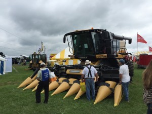
There were a variety of agriculture machinaries showing on the grass land. The farmers could conveniently talk to the dealers, in order to know more about the strength of these machinaries.

IMG_5351 IMG_5392

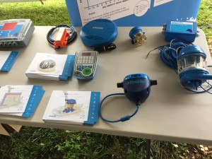
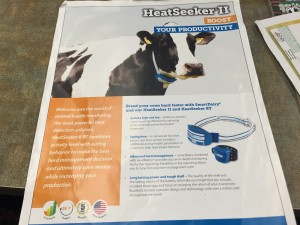
Also, there were a diversity of agriculture equipments that could be used to farm, keep livestock or market in a more convenient and precise way. I suppose that increasing use of such high-tech equipment must be a irreversible tendency nowadays.

IMG_5372IMG_5370

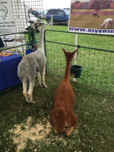
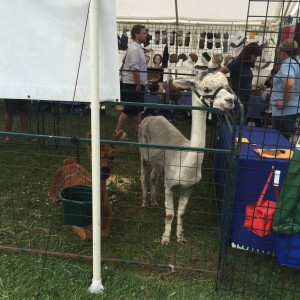
The most exciting thing for me was two alpacas. Before, I had only seen such cute animals on the websites, and I was so surprised to see that there’s a farm of alpacas in New York State. By the way, it’s interesting that these two alpacas showed their “somber” back to people from beginning to end.

I think this kind of event could definitely act as a great platform for local farmers to improve their knowledge, facilities and equipment that were useful for their farming work.

Skip to toolbar