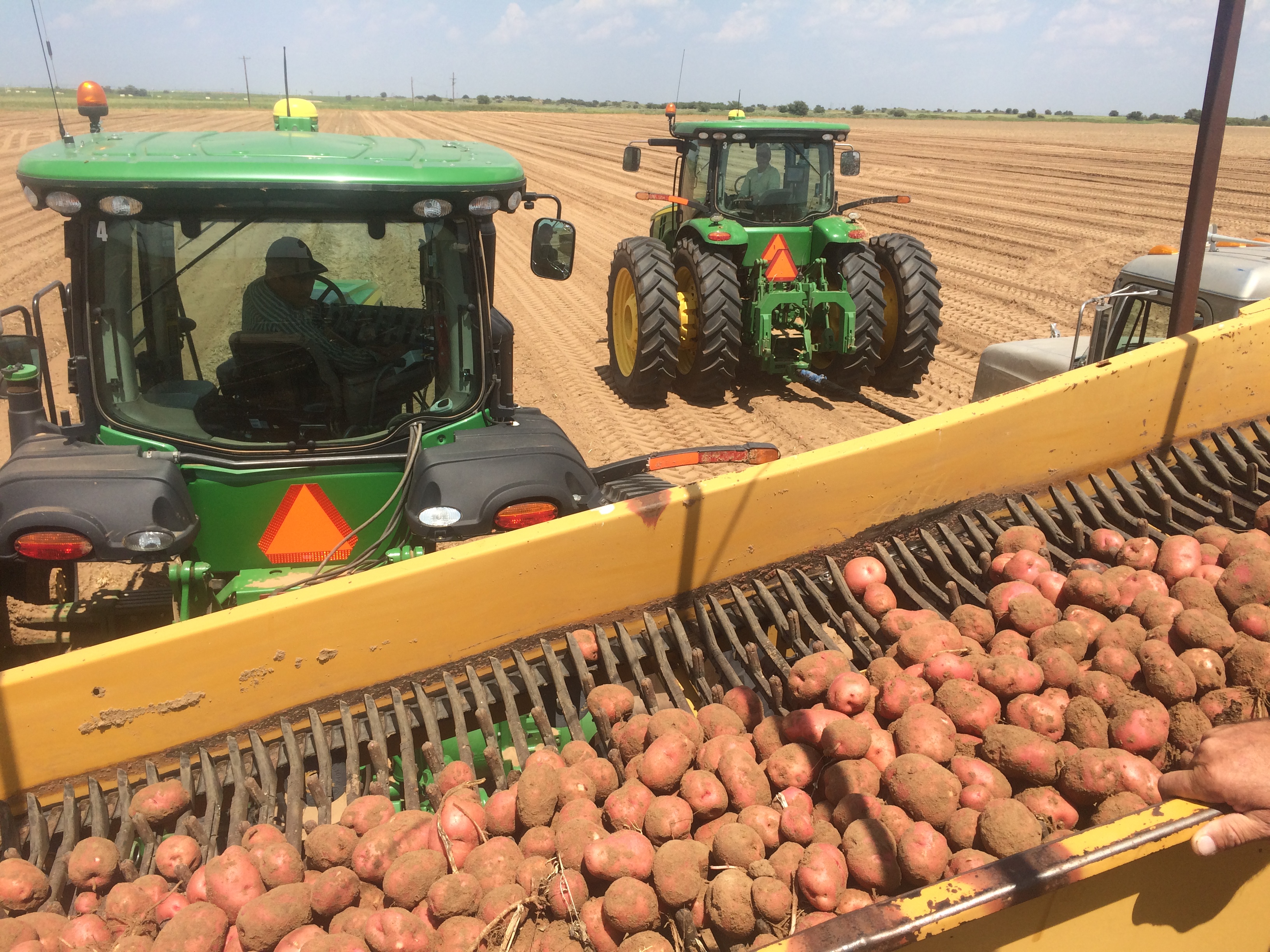
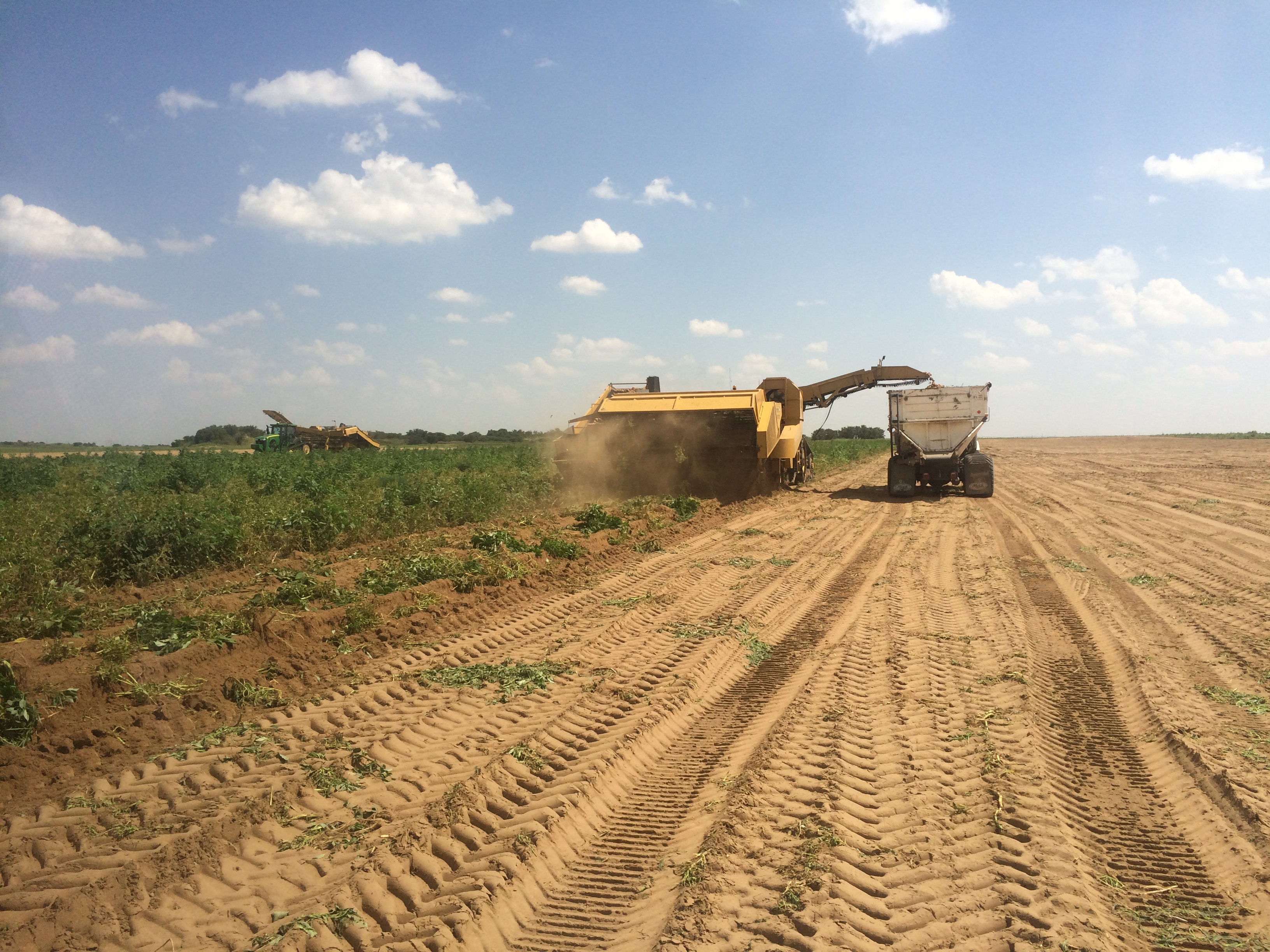
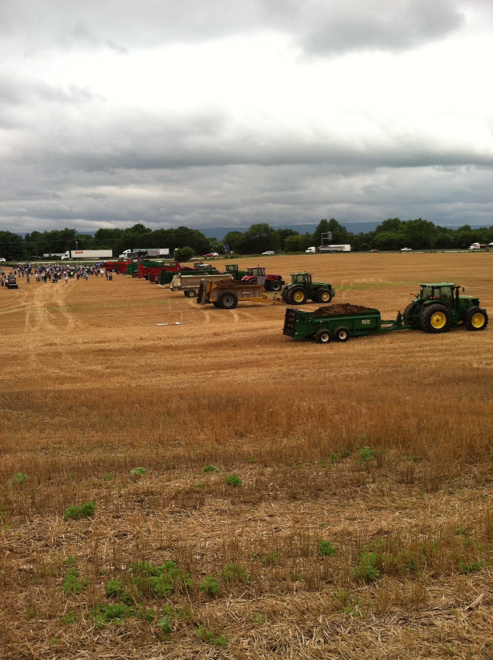
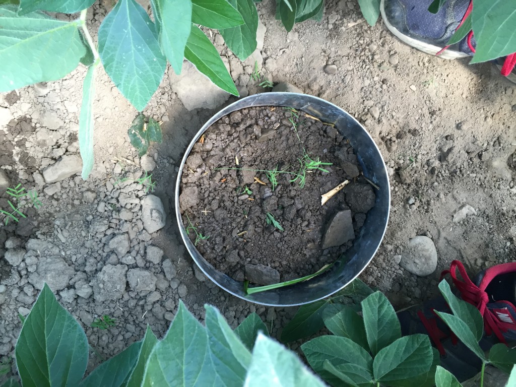
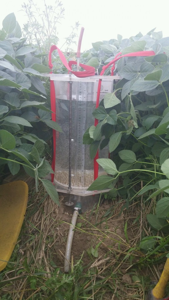
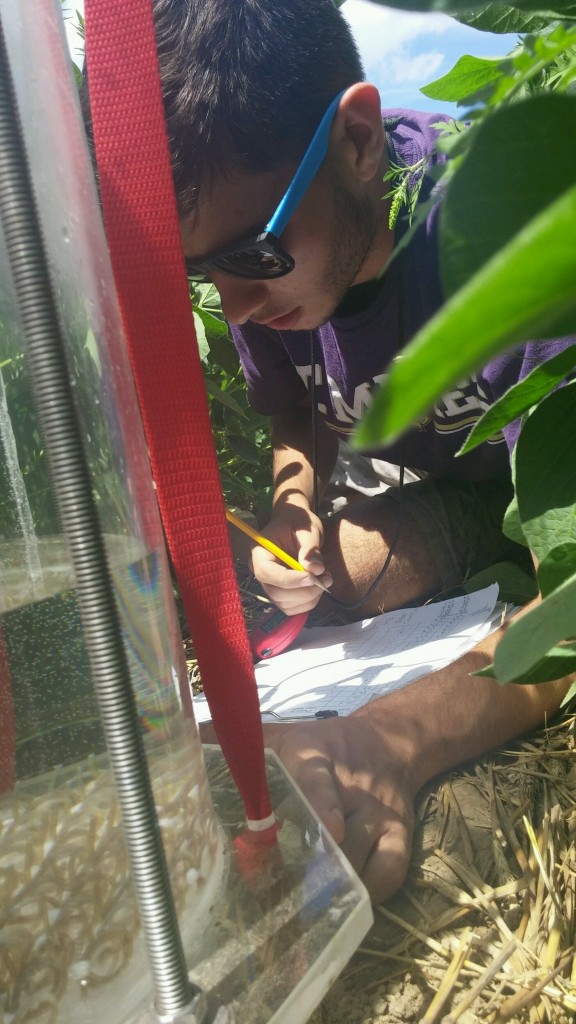
As part of my internship requirement for this summer, I partook in writing a two-page agronomy factsheet. Three students, including myself, wrote a factsheet following our internships during the Fall 2015 semester. We were able to write about any topic of our interest (since I worked with manure injection this summer, I decided to write about liquid manure injection). The coursework entailed meeting weekly as a group during the semester for approximately an hour and a half to two hours with additional hours of individual work (research, editing, formatting, etc).
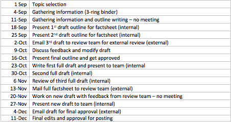
Schedule of weekly meetings
We each constructed an outline to organize our research into a order and manner that portrays our ideas logically. After weeks of gathering research and critiquing each other’s factsheets, Quirine Ketterings, who led the factsheet meetings, assembled a team of reviewers relevant to our topics to comment and edit (tare our outlines apart seemed to be the more accurate phrase) our factsheets.
After (surviving) the revisions for the outlines, we created our first drafts of our factsheets, and with a few more weeks of critiquing, editing and formatting, our papers were ready for another round of comments and edits from our review teams.
Once we survived the last round of edits, we each assembled awesome papers with insight into providing farmers in the state of New York with knowledge that will help their operations increase production and become more environmentally friendly.
Overall, I thoroughly enjoyed writing the factsheet. Between researching, receiving feedback from the review team and working with the equipment over the summer, I learned a tremendous amount of information about manure injection.
Here is link to my factsheet: http://nmsp.cals.cornell.edu/publications/factsheets/factsheet87.pdf