J.H. Cherney1, D.J.R. Cherney2, and M. Davis3
1Section of Soil & Crop Sciences, 2Dept. of Animal Science, Cornell University, and 3Farm Manager, Cornell Willsboro Research Farm, Willsboro, NY
Over five million acres of marginal agricultural land in the Northeast USA are no longer in use and have great opportunities for grass biomass production, although environmental or other supplemental compensation may be required for profitable production on low-yielding marginal land. Warm season grasses are considered a viable herbaceous second generation biofuel feedstock but are better suited to marginally productive cropland Future selection through breeding should have a significant focus on low-input types of environments.
Additional environmental benefits may accrue when mixtures are used instead of monocultures. Studies have suggested that polycultures sequester more carbon in the soil profile and have less N leaching compared to monocultures. Profitability in biomass production, however, is most strongly influenced by yield, and we focused on yield potential in this study.
Experimental layout
A long-term plot study was sown in 2010 in Ithaca (central NY, Williamson fine sandy loam soil) and Chazy (northern NY, Roundabout silt loam soil), and was completed in 2018. A goal was to determine if binary mixtures of warm-season grasses would result in increased yield over pure stands.
Three replicates of 12 treatments compared pure species with binary mixtures (Fig. 1). Binary mixtures had one species seeded in one direction, and the second species seeded perpendicular to the first. Pure species also were seeded twice, with one half the total seed sown perpendicular to the other half. Pure switchgrass and Atlantic coastal panic grass plots were seeded at 10 lbs pure live seed (PLS)/acre. Pure big bluestem plots were seeded at 12 lbs PLS/acre. Mixtures contained half the seeding rate of pure species plots for each species in a binary mixture. All entries were commercially available varieties, with the exception of RC Big Rock switchgrass, which was an experimental selection from Cave-In-Rock (REAP-Canada, Ste-Anne-de-Bellevue, QC). Insufficient seed was available of Timber switchgrass to seed at both sites.

Plots (15’ x 15’) were fertilized with 50 lbs N fertilizer/acre at spring green up each year. Roundup was sprayed in the spring prior to warm season grass green up to control weeds after 2013. A few weeds were resistant to Roundup and remained, such as milkweed. Plots were well established by the 2013 growing season. Plots were harvested for yield determination each year in early October generally after first frost at a 4” stubble height using a flail harvester, harvesting 78 sq. ft. of plot area (3’ x 13’ twice per plot). Samples were collected for dry matter (DM) determination.
Yield
The more southern, generally wetter, Ithaca site averaged 22% greater yield across all years and species combinations. Ithaca long-term average precipitation is 4.5” per year more than Chazy (Plattsburgh, NY weather station), and Ithaca averaged 5.5” more per year during the experiment. Although Chazy is considerably farther north than Ithaca, long-term average heat units are very similar. Over the 2013-2017 period from May 1 to Oct. 1, both sites averaged 4916 GDD per growing season (base 32F). Warm season grass mixtures behaved differently on different sites. At Chazy, big bluestem (BB) tended to compete very well in mixtures with switchgrass (SW), while at the Ithaca site switchgrass tended to be the major component.
Big bluestem was the slowest species to become fully established, but Prairie View BB pure stands were the highest yielding at the Chazy site, averaged over five years. RC Big Rock switchgrass selection had the greatest yield in Ithaca for pure SW stands, averaging 6.6 tons DM/acre over 5 years. Cave-in-Rock SW (CAV) and the CAV-Prairie View BB mixture both yielded 13% less at Chazy than Ithaca, but pure Prairie View stands produced similar yields at both sites. Upland switchgrass mixed with Prairie View BB tended to produce the best overall results and was the most compatible mixture (Fig. 2). Other mixtures tended to become mostly monocultures over time.

Atlantic coastal panic grass (ACP) was promising the first year, but quickly deteriorated to a weak stand after the first year, and had significant weed invasion in later years, particularly at Chazy. BoMaster switchgrass struggled in pure stands and became a very minor component of mixtures. In later years, big bluestem and switchgrass tended to invade plots with weaker stands, as ripe seed was scattered each year during harvest with a flail harvester.
Mixtures
At both sites, mixtures of Cave-in-Rock SW and ACP quickly became pure switchgrass stands. By the end of the trial, mixtures of Cave-in-Rock and Suther BB were pure switchgrass at Ithaca, and averaged 10% BB at Chazy. BoMaster SW and ACP, as well as mixtures of these two, tended to be weak stands at both sites, with up to 25% weeds observed in the summer of 2018. Prairie View BB and BoMaster SW mixtures were essentially pure big bluestem stands in 2018 at both sites. Suther BB and Cave-in-Rock SW mixtures were pure switchgrass in Ithaca, and averaged 10% big bluestem in Chazy. Prairie View BB and Cave-in-Rock SW mixtures averaged 15% bluestem in Ithaca and 35% bluestem in Chazy, at the end of the trial.
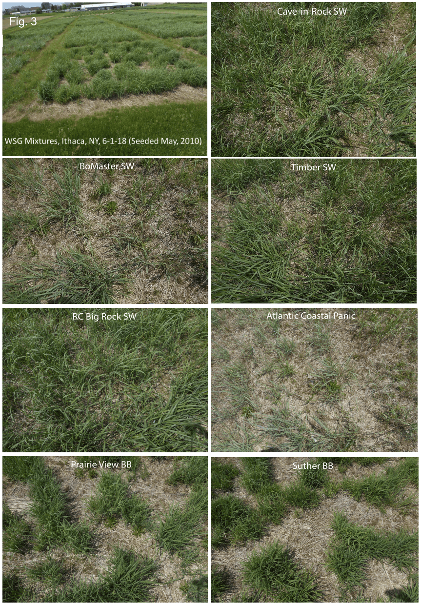
Ground cover
Plots in Ithaca were observed for ground cover in the spring of 2018 (Fig. 3). The three replicates were very consistent in ground cover. Switchgrass provided the most ground cover early in the season, with RC Big Rock SW appearing to have the greatest ground cover. BoMaster was the weakest switchgrass, typically with weed infestations. Approximately 50% of the ground area was bare in BB plots, but open areas were generally free of weeds. Even less surface area was covered by ACP, and open areas tended to be infested with weeds annually. With the exception of ACP at both sites, and BoMaster SW at Chazy, other species and species combinations developed into a closed canopy by mid to late summer, regardless of the ground cover observed in spring.
Summary
The only mixtures with a significant contribution from both species were Prairie View BB and Cave-in-Rock SW mixtures. These mixtures had considerably more switchgrass at the Ithaca site compared to the Chazy site. Our results agree with other studies suggesting that species mixtures will be largely influenced by environmental variation. Results from a single location may not be applicable to other environments. Mixtures can improve yields mainly in the establishing years, with the potential for better yield stability over the life of the stands. Farmers should consider planting adapted cultivar mixtures of big bluestem and upland switchgrass for enhanced yield and yield stability. Improving seedling establishment of big bluestem should be an important breeding priority for more widespread adoption of this crop.
Acknowledgments
This work was supported by the USDA National Institute of Food and Agriculture, Multistate project 218756. Any opinions, findings, conclusions, or recommendations expressed in this publication are those of the authors and do not necessarily reflect the view of the National Institute of Food and Agriculture (NIFA) or the United States Department of Agriculture (USDA).