Tulsi Kharel, Sheryl Swink, Connor Youngerman, Angel Maresma, Karl Czymmek, and Quirine Ketterings Cornell University Nutrient Management Spear Program
Calibration of yield monitors during the harvest season is essential for obtaining accurate yield data but even if calibrated properly, the data obtained from the yield monitors still need to be “cleaned”. Yield monitor values recorded are estimated based on:
Distance (inches or feet) travelled by the harvester during data logging time period.
Width (inches or feet) harvested during each logging time period.
Silage or grain flow (mass) measured by the equipment’s flow sensor per logging time period (lbs/second).
Moisture content (MC in %) of the harvested mass as measured by a moisture sensor per time period.
Logging interval of the yield monitoring system (seconds).
Errors that impact the accuracy of the yield data occur in multiple ways. The distance the combine/chopper travels during a time period and the width give the area required for yield calculation. If a combine is not equipped with a harvest swath width sensor, the default will be the chopper/combine width and that can cause errors when fewer rows are harvested than the equipment width. Another source of error is the delay time of grain or silage moving from the chopper/combine head to the flow rate sensor. Flow rate sensors, moisture sensors, and Global Positioning System (GPS) units are located in different places on harvest equipment and since it takes some time for harvested silage or grain to travel to the sensors, adjustments need to be made (this is called delay time correction). Each harvest pass will be affected by this delay correction, independent of whether a new pass starts from one end of the field or from somewhere within the field (in situations where the harvester is paused during harvest). The delay time itself is related to the speed of the combine/chopper as well, which may introduce another source of error.
Combines and forage choppers are calibrated for a certain velocity range. If the velocities that are recorded fall outside the calibrated range, flow rate and yield values associated with those points are no longer trustworthy and should be removed from the data. Similarly, abrupt changes in velocity affect the flow rate, resulting in erroneous yield calculations for logged data points. Other easily trackable errors are logged data points with zero grain or silage moisture; this may occur as the chopper or combine enters the field or pauses mid-field while the silage or grain flow has not yet reached the moisture sensor.
Last but not least, if the operator does not raise the combine/chopper head after completion of a pass, the pass number will not be updated in the logged dataset. Cleaning of data that are obtained this way will take additional effort, so lifting of the combine/chopper head while turning in the field is recommended.
The use of raw data without proper cleaning can lead to substantial over- and under-prediction of actual yield depending on the field and harvest conditions, especially for corn silage yield data. Figure 1 shows this in more detail for a number of fields. Look at a 20 ton/acre corn silage yield (cleaned yield) for the fields in this figure, and you will see that the raw data corresponding to this cleaned yield can range from 15 to 37 tons/acre! The raw data for many of the fields in this figure overpredicted yield, while for a number of other fields it actually underpredicted. Thus, data cleaning is absolutely necessary.
Figure 1: Not cleaning yield monitor data can result in large over or under predictions of actual corn silage yield.
In the past months, the Cornell Nutrient Management Spear Program, in collaboration with colleagues at the University of Missouri, the United States Department of AgricultureAgricultural Research Service (USDA-ARS) Cropping Systems and Water Quality Unit, Columbia MO, and the Iowa Soybean Association, evaluated cleaning protocols to develop a standardized and semi-automated procedure that allows for cleaning of datasets for whole farm yield data recording. The protocol developed for whole-farm data cleaning calls for unfiltered or “raw” harvest data files that are downloaded from the yield monitor with corresponding field boundary files. These files are read into the Ag Leader Technology Spatial Management System (SMS) software to preview the yield map and reassign any harvest data that might show up in the wrong field. Next, the individual field harvest data are exported as Ag Leader Advanced file format. The yield map files are then imported into Yield Editor (https://www.ars.usda.gov/research/software/download/?softwareid=370) for cleaning. Yield Editor is a freely available software developed by the USDA-ARS. The software allows for use of different ‘filters’ to remove the errors mentioned above. The final step in the cleaning protocol is deletion of data points with a moisture content <1 % for corn grain and <46 % for corn silage, which can be done in Yield Editor or in MS Excel or other sortable spreadsheet program. This final step is particularly important for obtaining accurate corn silage yield data. A step-by-step protocol for cleaning individual field datasets and batch processing of harvest data from growers with large numbers of corn silage or grain fields is described in a manual that is available for downloading from the YieldDatabase page (http://nmsp.cals.cornell.edu/NYOnFarmResearchPartnership/YieldDatabase.html) of the Cornell Nutrient Management Spear Program website.
Farmers with an interest in sharing corn silage and/or grain yield data with the Nutrient Management Spear Program for updating of the Cornell University yield potential database are invited to get in touch with us. The protocols for data sharing are available at the same weblink listed above. If interested in training sessions on the cleaning protocol this winter, contact Quirine M. Ketterings at qmk2@cornell.edu.
Acknowledgments
We thank the farmers and farm consultants that supplied data for this project, and our NMSP team members and colleagues in Missouri and Iowa for working with us on the protocol. For questions about the project contact Quirine M. Ketterings at 607-255-3061 or qmk2@cornell.edu, and/or visit the Cornell Nutrient Management Spear Program website at: http://nmsp.cals.cornell.edu/.
Savanna Crossman, Precision Agriculture Research Coordinator New York Corn and Soybean Growers Association
The 2016 field season marked the first year of testing for the variable rate planting model that is being developed by the Precision Ag Research Project. Growers across New York State know the challenges that the severe summer drought brought to our region. Crop yields were impacted across the state and the research was no exception. While unfortunate, it is advantageous to be able to test the model during a dry year and learn from how the crops reacts to the stress.
Across the board, the mid-to-lower seeding rates fared the best in the corn and soybean trials. The model was tested on five fields this year and only four made it to grain harvest due to severe drought stress. The results revealed that in three of the fields, there was not a significant difference in the profit produced by the model. While the average yield of the model was significantly less, the model was able to achieve similar profit per acre by using lower seeding rates. (Table 1)
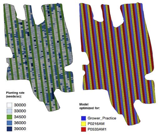
Figure 1. 2016 Beach 2 model design. The left image displays the planting rate map and the right image displays the hybrid map.
A variation of the model design was planted on one field, Beach 2, in a split planter fashion with two contrasting hybrids. This varied design was used as it allowed for of multiple points of comparison, including hybrid comparison. Check strips were integrated every two passes to allows direct comparison of how the model performed to the typical grower practice rate. From there, the design becomes more complicated. The first pass would be planted at the model optimized rate for hybrid A, which meant hybrid B was also being planted at that same rate. Then the next pass would plant at the rate optimized for hybrid B while hybrid A was being planted at that rate as well. This allows us to examine the hybrid response to population in more depth. (Figure 1)
The hybrids P0216 and P0533 were selected due to their differences in plant architecture and responses to stress. In years of excellent growing conditions, the tight leaf structure and short stature of P0533 will produce aggressive yields. The hybrid P0216 will produce average yields in years of stress as well as in excellent conditions.
A 4,000 foot view of this field would show that there was not a significant yield difference between the model and the grower’s flat rate. The model yielded about 2 bu/ac more than the flat rate, but that difference was not statistically significant. When we separate the results out by hybrid, we see a much more telling story.
These hybrids resulted in a wonderful side-by-side comparison this year. When compared to the flat rate, P0533, regardless of optimization, yielded significantly more per acre and yielded an astounding $64/ac more. Conversely, P0216, regardless of optimization, yielded less than the flat rate and produced a profit $22/ac less than the flat rate.
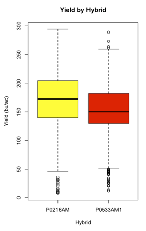
Figure 2. P0216 optimized yield versus P0533 optimized yield.
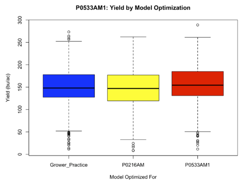
A deeper look into the results showed that that when both hybrids were planted optimally, P0216 yielded almost 18 bu/acre higher than P0533 (Figure 2). It also demonstrated that P0533 exhibited a statistical significant response to model optimization. Meaning, when it was optimized the yield significantly improved over not being optimized (Figure 3). This is likely due to the fact that in a stressful year, P0216’s yields will not fall apart due to seeding rate while P0533 benefited from precise placement.
Figure 3. P0533 exhibited a hybrid response to population.
These same hybrids in Beach 2, however, exhibited the exact opposite hybrid response in 2014 which was a normal year in terms of weather conditions. Knowing this emphasizes the importance of multiple years of testing and data collection to create a robust algorithm. The biggest gain from the 2016 season has been the strong design and analysis process that has been developed. What the project has accomplished in these terms, is at the leading edge of the scientific community.
In order to build upon what the project has already accomplished, the project is still looking to get more producers involved and participating. The project aims to get fields in the research that have a large amount of variation and are fifty acres or greater. Any interested growers are highly encouraged to get in touch with the Project Coordinator, Savanna Crossman, at 802-393-0709 or savanna@nycornsoy.com.
Rintaro Kinoshita1, Aaron Ristow1, Harold van Es1, John Dantinne2, and Michael Twining3
1 Soil and Crop Sciences Section, Cornell University; 2Millersville PA, 3Willard Agri-Service, Inc.
Background Digital agriculture is a new concept that focuses on the employment of computational and information technologies to improve the profitability and sustainability of agriculture. A promising opportunity is the use of advanced analytical methods on data that are routinely collected on farms, which allow insight into ways to improve management. One example is the use of combine yield monitor data that are now customarily collected as part of harvest operations.
Crop fields have high variations in crop performance due to varying soil types and topography, which interact with climate and management. A major objective of most growers is to maximize profit. Understanding the underlying profitability potential in varying areas of agricultural fields allows managers to construct zone-specific strategies using information on yield potential and yield-constraining factors.One might consider two management interventions to optimize profitability: (i) take field areas that are known in advance to be unprofitable out of crop production, and (ii) make underperforming field areas more profitable through improved management implementation.
Therefore, our objectives were to (i) evaluate the variation in spatial patterns of within-field profitability as well as field-average expected profitability, and (ii) determine opportunities for site-specific management change to increase overall field profitability.
Procedures The study fields are located in Delaware, Maryland, Virginia, West Virginia, and southeastern Pennsylvania within three physiographic provinces: Coastal Plain, Piedmont, and Blue Ridge. All fields had similar crop rotations: corn, soybean, and wheat or barley. In some cases, double crop soybean was cultivated following the harvest of small grains. Soil nutrient, pest, weed, and irrigation water management on each field was based on individual farm’s management schemes.
Yield data were collected for corn and soybean on 18 fields throughout the study region with well-calibrated yield monitors on combine harvesters. The fields ranged in size from 14.3 to 115.9 acres. For a particular field, the number of growing seasons for which digital yield data were available ranged from 3 to 12, with a range of 1 to 7 growing seasons for a single crop. Irrigation occurred on 6 of the 18 fields. Post-processing of yield data was done using the Yield Editor 2.0.7 software and data were then rasterized (15×15 ft) using the SAGA function within the QGIS environment.
We calculated site-specific profitability using:
Profitability = E[Yield]xPrice – Cost (1)
where E[Yield] is the expected value of yield estimated from the multi-year average yield, Price is the average price of the crop (corn or soybean), and Cost is the average cost of production. We utilized the 10 year average (2004-to-2013) price of corn and soybean for the profitability calculation, which were $4.73 and $411.45 per bushel, respectively (University of Illinois, 2015). The cost of production was determined using the Farm Resource Regions (USDA-ERS, 2000) for 2014, and ranged from $590.6 to $666.7 per acre for corn and $395.3 to $437.0 per acre for soybean.
We adopted different scenarios for profitability calculation for both rented and owned fields, where we subtracted the land rental rate from the total cost. We also estimated the cost of irrigation to be $138.0 per acre (Tyson and Curtis, 2008), which was added to the total annual cost of production when appropriate.
Results and Discussion
Field-Scale Profitability In the first analysis, the variation in spatial patterns of within-field profitability as well as field-average expected profitability was evaluated. Expectedly, profitability was affected by owned versus rented field status (Table 1) in both corn and soybean scenarios. In the owner-field scenario, 76% of the field area was on average profitable compared to 57% for the rented scenario. Profitability was higher overall in soybeans compared to corn for both owned and rented scenarios, partly due to the assumed lower cost of production by approximately $200 per acre (USDA-ERS, 2015) and mostly related to the exclusion of N fertilizer cost.
Irrigation effectively improved profitability (not shown here), even under rented scenarios, indicating that soil moisture shortage is a major yield limiting factor in the Mid-Atlantic region and irrigation can achieve positive profits even after accounting for the added cost.
Spatial Patterns of Profitability and Opportunities for Alternative Land Uses A second analysis focused on the identification of profitable vs. unprofitable zones within fields. I.e., based on multi-year yield data, can we consistently expect certain parts of the field to be money losers? We identified three general categories of within-field profitability patterns: “economically sensitive” (Fig. 1a and 1b), “distinct profitable-unprofitable zones” (Fig. 1c and 1d), and “all-profitable” (Fig. 1e and 1f).
Fig. 1. Selected maps of within-field profitability for the owned-field scenario for corn representing three profitability categories; a and b) economically sensitive; c and d) distinct profitable-unprofitable zones; and e and f) all-profitable.
The economically sensitive fields generally showed high temporal variation in yield pattern due to irregular precipitation, and due to most areas being on average, either slightly profitable (Fig. 1a and 1b; green zones) or slightly unprofitable (yellow zones). This indicates that profitability at a field location strongly depends on the growing season’s environmental conditions and the relative prices of inputs and grains. The small margins in profitability suggest that modest changes in production efficiencies, grain prices, input costs, or localized yields can turn areas from unprofitable to profitable, or vice versa. For example, in fields 1a and b most profitable green zones would turn unprofitable with a $0.50 drop in grain prices. Conversely, reducing fertilizer costs through precision N management could change yellow zones from unprofitable to profitable.
In fields with distinct profitable-unprofitable zones, areas exist that are either consistently profitable or unprofitable (Fig. 1c and 1d). The profitable areas (light and dark blue) presumably have favorable growing conditions, while the consistently unprofitable areas of the fields (orange and red) experience yield-limiting conditions. In some fields, money-losing zones of $200 per acre (red) existed along with $200 per acre money-making zones (blue), resulting in a $400 per acre total profitability range. The very profitable areas in these fields have higher than field-average yield potential, which may warrant increased site-specific inputs like fertilizer and possibly seed.
The consistently low-yielding zones are possibly compacted headlands, areas experiencing shading from adjacent woods, damaged by wildlife, erosive or poorly-drained. Since profitability for those field zones is predictably negative, overall field profitability would be enhanced by taking those field areas completely out of production. For example, herbaceous buffer strips on the field borders or in swales could be installed to enhance environmental benefits while still providing equipment turnaround space and minimal effects on yield in the rest of the field. We evaluated the removal of low profitability areas (< -$200 per acre) from the field in Figure 1c and found an increase in overall field profitability from $41 to $63 per acre.
Alternatively, potential areas of yield-constraining factors, like compaction, poor drainage or low organic matter, may be identified and managed to make those field areas profitable. For example, season-specific yield constraints were identified for the two fields in Figure 1d from excessive early-season precipitation combined with poorly-drained soil from concave field areas. Over time, improving the soil health status of these areas could make them profitable.
A third profitability pattern shows field areas being all profitable (Fig. 1e and 1f). These are the most preferred conditions where no additional considerations are warranted and fields can be managed uniformly.
Conclusions Adoption of yield monitoring has accumulated large amounts of data. Based on our analysis of multi-year site-specific data, yields vary spatially and temporally at the field scale. We assessed within-field spatial patterns of profitability using grower collected yield data and input cost information for fields in the Mid-Atlantic USA. Three types of profitability pattern categories were identified: economically sensitive, clear profitable-unprofitable zones, and all-profitable. For fields with areas of permanent yield constraints, the removal of consistently unprofitable areas can increase overall field profitability. Conversely, high-yielding zones may justify more inputs, notably higher fertilizer and possibly seed rates. Other fields showed high sensitivity to prices and may benefit from improved management efficiencies. In conclusion, the combination of site-specific profitability and yield constraint information can inform future management optimization, including removing field areas from crop production entirely and improving management efficiencies.
Acknowledgements We are grateful to the participating growers for providing the yield data. This work was supported by grants from Willard Agri-Service, Inc., the New York Farm Viability Institute and the USDA-NRCS.
References Kinoshita, R., H. van Es, J. Dantinne and M. Twining. 2016. Within-Field Profitability Analysis Informs Agronomic Management Decisions in the Mid-Atlantic, USA. Agricultural and Environmental letters. 1:160034. doi:10.2134/ael2016.09.0034.
Tyson, T.W., and L.M. Curtis. 2008. 60 acre pivot irrigation cost analysis. Department of Biosystems Engineering, Auburn Univ., Auburn.