The Impact of the Use of Greater Money Values in the Ultimatum Game
In Friday’s lecture (9/21/12) we discussed the “Ultimatum Game” and its applications to analyzing the impact of power in social networks. The basic premise of the game is that a person A is given an certain amount of money and is expected to offer a fraction of that money (of A’s choosing) to person B. Person B can then either accept or reject that offer. If B rejects it, neither player receives any money, however if B accepts it, both A and B receive the money dictated by the terms of A’s offer. Therefore there is some incentive for A to use his or her intuition in proposing an offer that B will accept, but also result in A keeping a larger share of the money. In class using iClickers we obtained a simple distribution of offers by A to divide up $10. There was an interesting split, a large number of students chose to offer $5, while another fairly large number of students chose to offer $1. In practice, scientific studies have found it difficult to obtain large amounts of data on the rejection and acceptance of low offers.
In an attempt to increase the sample size of low offers, a 2011 study by Anderson et al. that appeared in the American Economic Review journal, made a slight change to the game. In their instructions to the participants of the study they provided an explanation of the “rational” choice that results in participants walking away with the most money at the end of the experiment. The person being offered money should accept any amount proposed in the ultimatum, while the person offering the money should attempt to keep as much money as possible (since they should expect the other person to accept nearly any offer). Their findings indicate that this slight change in the game gave them the results they were looking for.
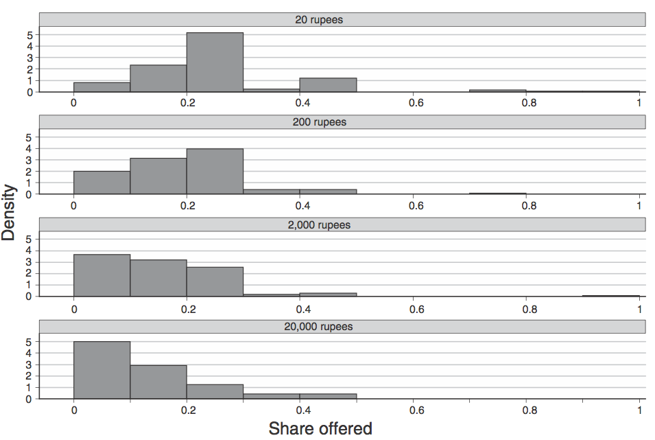
We saw in class that a fairly large proportion of students chose to offer 50% of the pool of money. In the case of the study, with the modification to the game, the offerers tended toward lower proportions even in the lower stakes cases. As a reference, the study states that 20 rupees corresponded to about 41 cents at the time and 1.6 hours of work. In our society $10 corresponds to a little more than 1 hour of work. Therefore the results of our quick iClicker experiment would be somewhat analogous to the 20 rupee experiment conducted in the study. The 20 rupee game resulted in only a little more than 1/5 of the offers coming in at above 40% of the pool. Most offers were between 10 and 30%. In our experiment a higher proportion of offers were above 40%. The results for offer proportion at the different stakes levels of the Anderson et al. 2011 study are shown in the following figure.
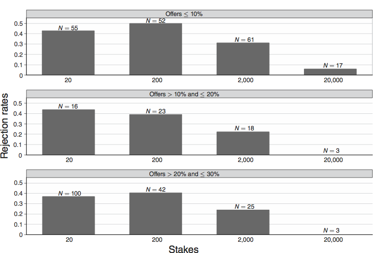
The main aspect of this study though was the impact of stakes on the rejection rates of low percentage offers. Figure 2 shows some of the results for the rejection rates at low offers at each stakes level (they used 20, 200, 2000, and 20000 rupees). Clearly as the stakes get higher (towards the 2000 and 20000 rupee range), the rejection rates drop relative to the lower stakes games. We can see that only one offer was rejected in the highest stakes game, and that came in at less then 10% of the total pot, so the overall rejection rate is extremely low as at high stakes. Oddly enough it seems as though the rejection rate for low offers in 200 rupee game was higher overall than in the 20 rupee game. No discussion or possible explanation was given for this, and perhaps it was because the difference could have been due to chance (in other words it was not statistically significant).
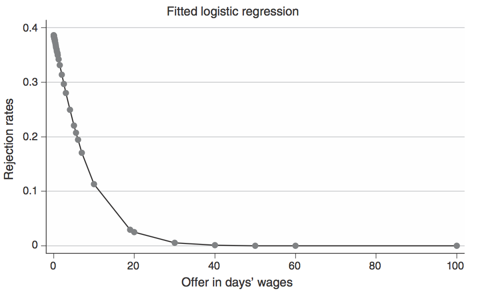
The change in the instructions of the game increased the number of low offers to the point where the authors of the paper were able to obtain enough data on rejection rates to fit a regression curve that could be used to predict how often someone would reject an offer as a function of the amount of money that was on the table (in this case normalized to represent the value as specific number of days worked so that it can be more readily applied to different economic climates since their study took place in a rural region of India).
In their analysis they found that the proportion of the total money offered was one of the most significant factors in determining the rejection rate. However they also found that there was a particular offer cutoff at which the participants accepted all offers (around 40 days worth of wages). Below that point there was still a chance that the offer might get rejected. This means that as the stakes get higher, the offerer can keep an increased percentage of the total money without the risk of their offer being rejected. The relationship they derived is depicted in Figure 3.
Something that was also considered in this experiment was the effect on wealth of the decision making of the participants. To test this they paid some participants for “unrelated tasks” prior to the experiment. Those who received this money were considered “wealthy.” The study found little impact of wealth on the decision making of the participants to accept or reject offers. In other words it was not determined significant in their regression analysis model for rejection rates. So really what was at play in these games was the gut feelings of the participants, not something rational like how much money they had.
Overall, we can see that we get drastically different results as the stakes of the game change. Therefore it is something to keep in mind when developing our intuition about games. There comes a point when people will put their feelings aside and accept an offer, however unfair, if the payoff is great enough for them. In India, it appears that this strict cutoff is at 40 days of work, but rejection rates drop rapidly between 0 and 20 days work (dropping below 10% at around 15 days). Finally, these results reflect mainly the gut feelings of the participants, because their initial payoff from the experiment (in the form of “wealth”) did not have a statistically significant impact on their decisions.
-_________


